支持向量机(SVM)

什么是支持向量机呢?支持向量机是监督机器学习模型,可对数据进行分类分析。实际上,支持向量机算法是寻找能将实例进行分离的优秀超平面的过程。
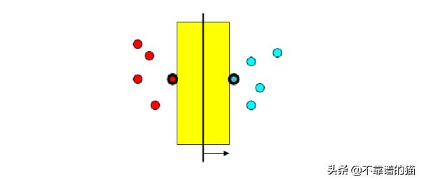
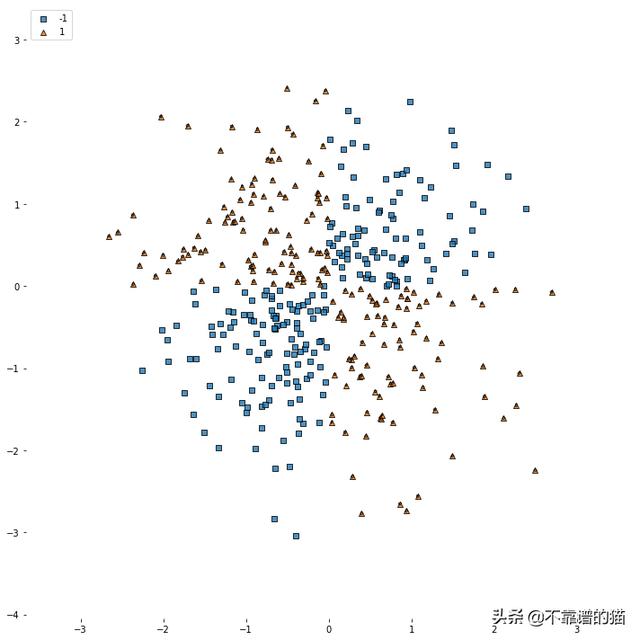
如果数据像上面那样是线性可分离的,那么我们用一个线性分类器就能将两个类分开。如果我们的数据是非线性可分的,我们应该怎么做呢?就像这样:
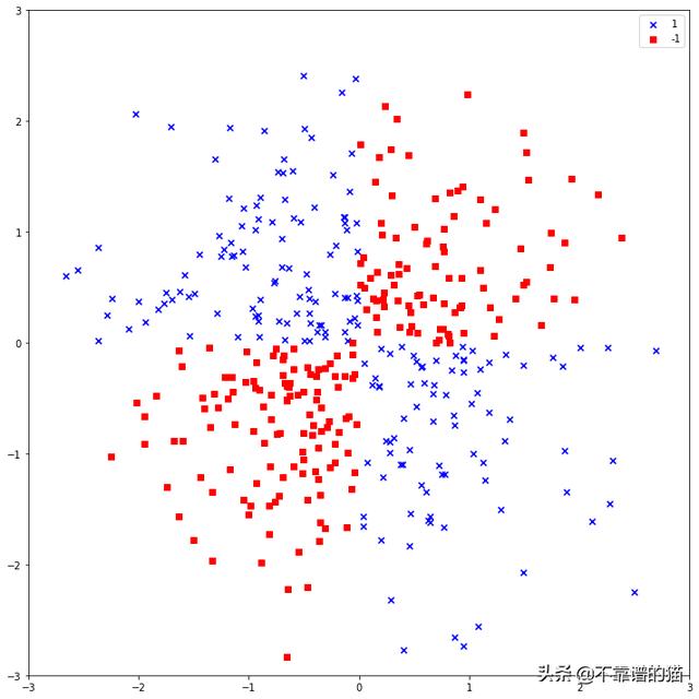
正如我们所看到的,即使来自不同类的数据点是可分离的,我们也不能简单地画一条直线来进行分类。
那么我们如何使用支持向量机来拟合非线性机器学习数据集呢?
使用SVM进行实验
创建机器学习数据集
首先创建非线性机器学习数据集。Python代码如下:
- # Import packages to visualize the classifer
- from matplotlib.colors import ListedColormap
- import matplotlib.pyplot as plt
- import warnings
- # Import packages to do the classifying
- import numpy as np
- from sklearn.svm import SVC
- # Create Dataset
- np.random.seed(0)
- X_xor = np.random.randn(200, 2)
- y_xor = np.logical_xor(X_xor[:, 0] > 0,
- X_xor[:, 1] > 0)
- y_xor = np.where(y_xor, 1, -1)
- fig = plt.figure(figsize=(10,10))
- plt.scatter(X_xor[y_xor == 1, 0],
- X_xor[y_xor == 1, 1],
- c='b', marker='x',
- label='1')
- plt.scatter(X_xor[y_xor == -1, 0],
- X_xor[y_xor == -1, 1],
- c='r',
- marker='s',
- label='-1')
- plt.xlim([-3, 3])
- plt.ylim([-3, 3])
- plt.legend(loc='best')
- plt.tight_layout()
- plt.show()
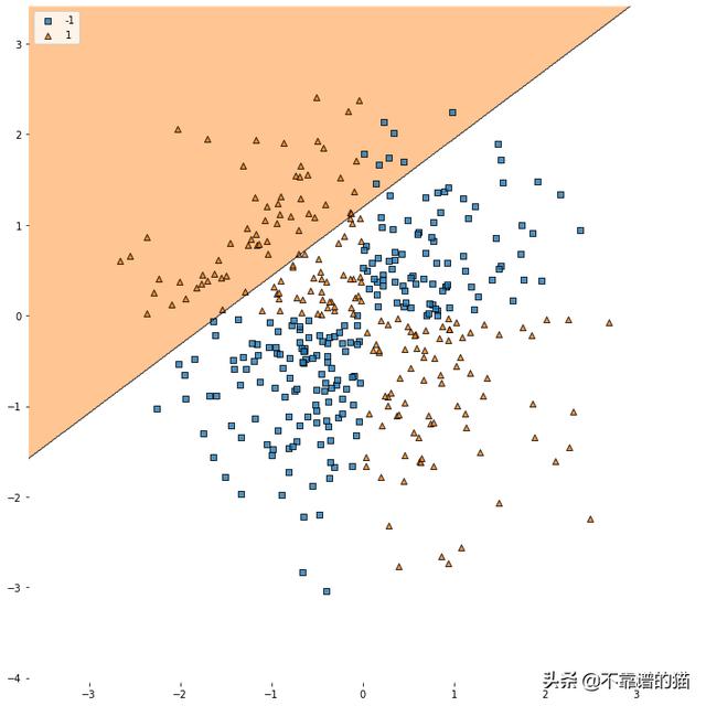
尝试使用线性支持向量机
我们首先尝试使用线性支持向量机,Python实现如下:
- # Import packages to do the classifying
- from mlxtend.plotting import plot_decision_regions
- import numpy as np
- from sklearn.svm import SVC
- # Create a SVC classifier using a linear kernel
- svm = SVC(kernel='linear', C=1000, random_state=0)
- # Train the classifier
- svm.fit(X_xor, y_xor)
- # Visualize the decision boundaries
- fig = plt.figure(figsize=(10,10))
- plot_decision_regions(X_xor, y_xor, clf=svm)
- plt.legend(loc='upper left')
- plt.tight_layout()
- plt.show()
C是与错误分类相关的成本。C值越高,算法对数据集的正确分离就越严格。对于线性分类器,我们使用kernel=’linear’。
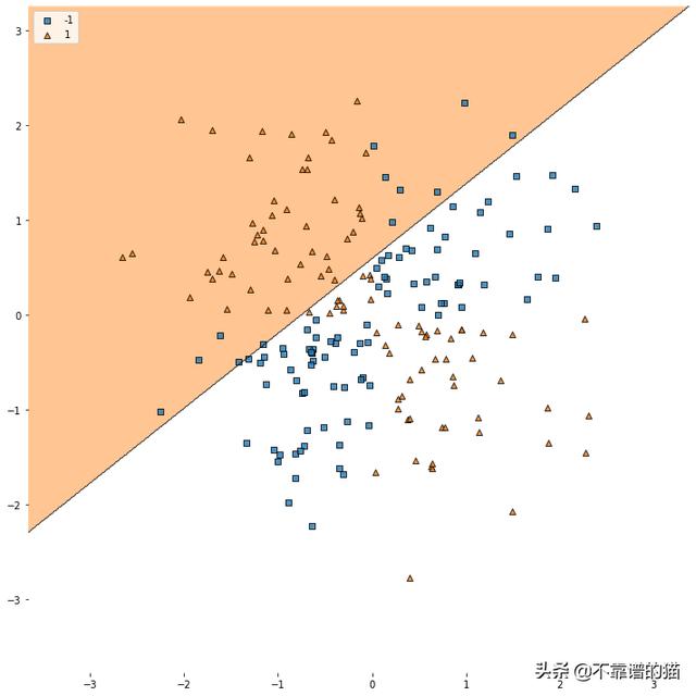
如我们所见,即使我们将成本设置得很高,但这条线也无法很好地分离红点和蓝点。
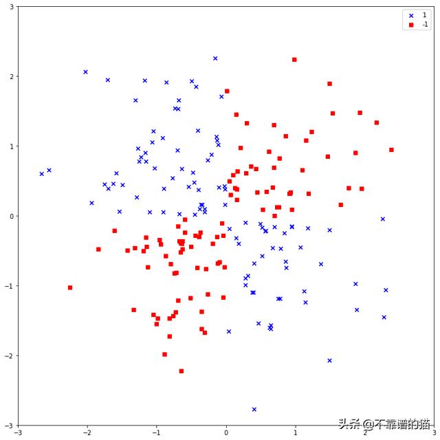
径向基函数核
到目前为止,我们使用的线性分类器为:
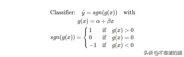
正如我们所看到的,g(x)是一个线性函数。当g(x) >为0时,预测值为1。当g(x) <0时,预测值为-1。但是由于我们不能使用线性函数处理像上面这样的非线性数据,我们需要将线性函数转换成另一个函数。
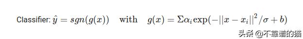
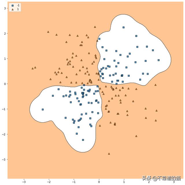
这个分类器似乎是我们非线性数据的理想选择。让我们来看看Python的代码:
- # Create a SVC classifier using an RBF kernel
- svm = SVC(kernel='rbf', random_state=0, gamma=1/100, C=1)
- # Train the classifier
- svm.fit(X_xor, y_xor)
- # Visualize the decision boundaries
- fig = plt.figure(figsize=(10,10))
- plot_decision_regions(X_xor, y_xor, clf=svm)
- plt.legend(loc='upper left')
- plt.tight_layout()
- plt.show()
gamma是1 / sigma。请记住,sigma是调节函数。因此,gamma值越小,sigma值就越大,分类器对各个点之间的距离就越不敏感。

让我们把伽玛放大看看会发生什么
- # Create a SVC classifier using an RBF kernel
- svm = SVC(kernel='rbf', random_state=0, gamma=1, C=1)
- # Train the classifier
- svm.fit(X_xor, y_xor)
- # Visualize the decision boundaries
- fig = plt.figure(figsize=(10,10))
- plot_decision_regions(X_xor, y_xor, clf=svm)
- plt.legend(loc='upper left')
- plt.tight_layout()
- plt.show()
好像将伽玛值提高100倍可以提高分类器对训练集的准确性。把伽马值再乘以10会怎么样呢?
- # Create a SVC classifier using an RBF kernel
- svm = SVC(kernel='rbf', random_state=0, gamma=10, C=1)
- # Train the classifier
- svm.fit(X_xor, y_xor)
- # Visualize the decision boundaries
- fig = plt.figure(figsize=(10,10))
- plot_decision_regions(X_xor, y_xor, clf=svm)
- plt.legend(loc='upper left')
- plt.tight_layout()
- plt.show()
这是否意味着如果我们将伽玛提高到10000,它将更加准确呢?事实上,如果伽玛值太大,则分类器最终会对差异不敏感。
让我们增加C。C是与整个机器学习数据集的错误分类相关的成本。换句话说,增加C将增加对整个数据集的敏感性,而不仅仅是单个数据点。
- from ipywidgets import interact, interactive, fixed, interact_manual
- import ipywidgets as widgets
- warnings.filterwarnings("ignore")
- @interact(x=[1, 10, 1000, 10000, 100000])
- def svc(x=1):
- # Create a SVC classifier using an RBF kernel
- svm = SVC(kernel='rbf', random_state=0, gamma=.01, C=x)
- # Train the classifier
- svm.fit(X_xor, y_xor)
- # Visualize the decision boundaries
- fig = plt.figure(figsize=(10,10))
- plot_decision_regions(X_xor, y_xor, clf=svm)
- plt.legend(loc='upper left')
- plt.tight_layout()
- plt.show()
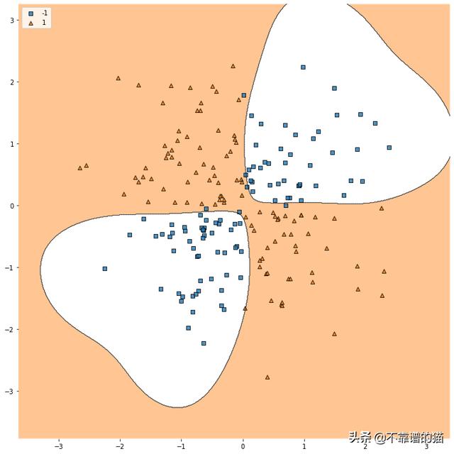
我们已经找到了参数,因此我们的SVM分类器可以成功地将两组点分开。
最后
我希望本文能让您对SVM分类器是什么以及如何使用它来学习非线机器学习性数据集有一个直观的认识。如果数据是高维的,您则无法通过可视化来判断分类器的性能。好的做法是根据训练集进行训练,并在测试集上使用混淆矩阵或f1-分数等指标。
作者:不靠谱的猫_今日头条
原文链接:https://www.toutiao.com/a6828957941589082628/
转载请注明:www.ainoob.cn » 如何使用支持向量机学习非线性数据集